vt.

Motivation

The notion for writing this blog came when I realized that everything that I learned was so cluttered inside my head and decided to write everything in a single space to anchor them together. This is not the first or last implementation of the same and by any means is unique, on the other hand, it's just my interpretation of the same and the main point is for it to be written more than to be read.

Idea

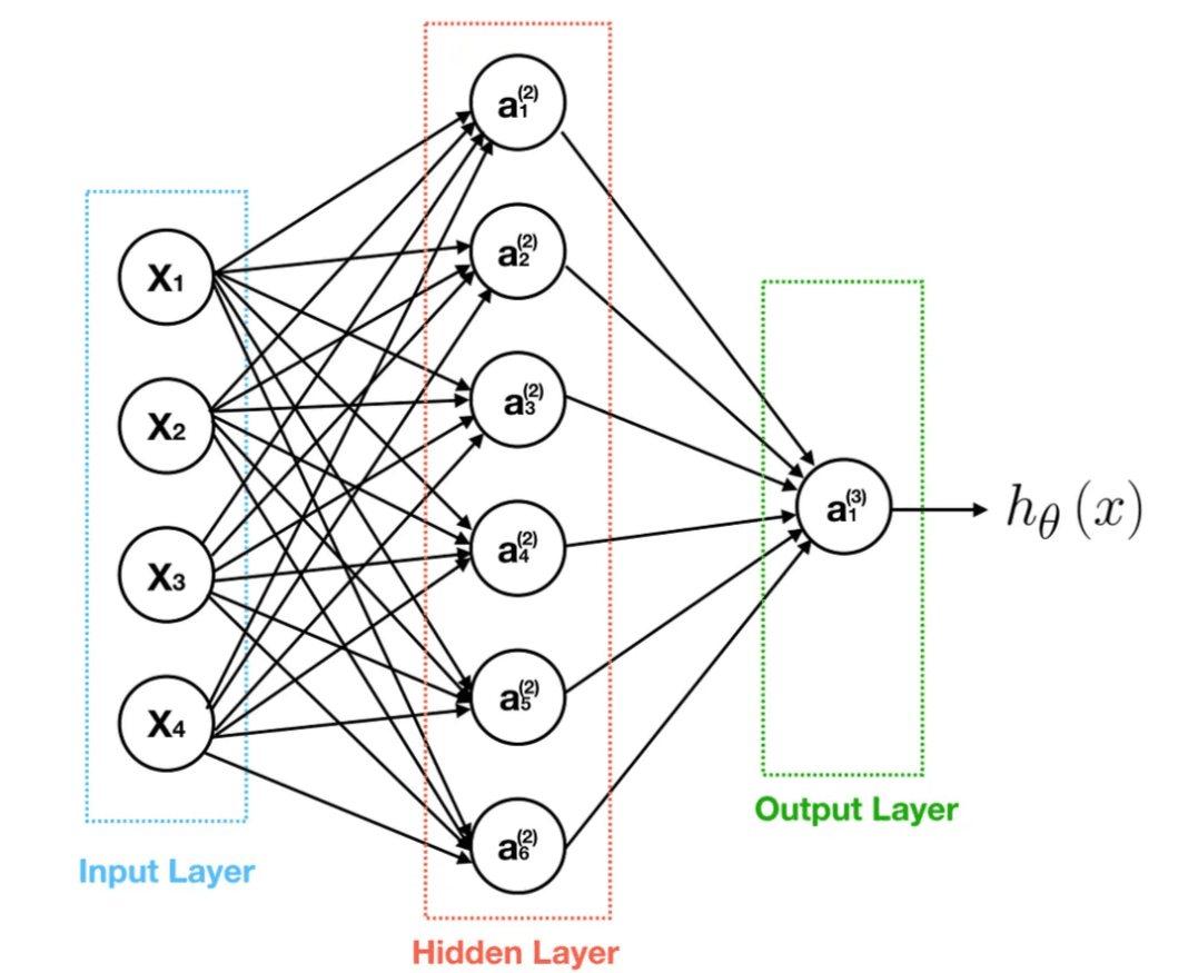
What is a neural network? - The first time was asked that, I thought it had to do something with biology (probably you did too). In practice, it has little to absolutely no relation with it. The only correlation is that the network comprises layers(called perceptrons) that consist of neurons(loose analogy from the human brain) that perform some operations on the data that is fed on to them. The different hidden layers when connected are termed as the neural network. A visual representation of the same-

Concept

Forward Propagation

For simplicity let us consider a neural network with only 2 layers. The input data is fed into the input layer or layer 1 of the model, for which each neuron calculates the value of a function called activation function (decides whether the neuron will be activated to contribute to the output) using a separate set of values for the weights and biases(used to optimize the value of the output) which are used in the function mentioned below and then appends the values

a_1,a_2,.....,a_n

into a new vector a.

Sigmoid\ Function: g(z) = \frac{1}{1 + e^{-z}}

z = w_j \cdot x + b

The graph for the function is:

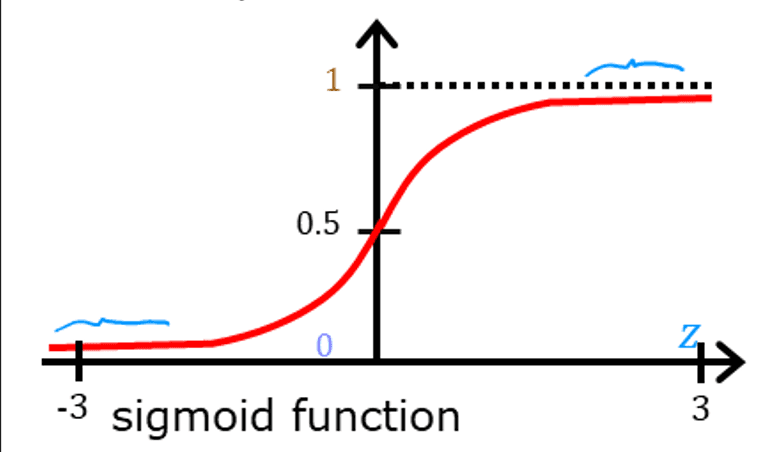
From the graph, it is evident that the reason for selecting the sigmoid function for logistic regression here is that it outputs values between 0 and 1 only. If z=0: g(z)=0.5, z>0: g(z) lies between 0 and 1 but approaches 0, z<0: g(z) between 0 and 1 but approaches 1. Therefore it is a perfect function for us to use when we need to classify output values between 0 and 1.

Continuing with the output of layer 1 as the vector a, which is the input for layer 2 (also the output layer). The output layer only has 1 neuron unit to simplify the vector input as a scalar output, computation for the activation output remains the same. The resultant scalar output is the final output of the network.

Cost Function

The output vector "a" is then compared with the actual value to find how well the output matches the target values. The difference between the target value and prediction is referred as loss for each value.

The loss function that we will be using is also called Binary Cross Entropy Loss and is the same one used in logistic regression for classification.

\text{Binary Cross-Entropy Loss} = -\frac{1}{2m} \sum_{i=1}^{m} \left[ y_{\text{true}}^{(i)} \log(y_{\text{pred}}^{(i)}) + (1 - y_{\text{true}}^{(i)}) \log(1 - y_{\text{pred}}^{(i)}) \right]

Back Propagation

To minimize the losses, an algorithm called gradient descent is used, which determines the value of weights(w) and biases(b). For gradient descent, we first find the average gradients over "m" training samples :

\frac{\partial L}{\partial w}= \frac{1}{2m} \sum_{i=1}^{m} \left( (y_{\text{pred},i} - y_i) \cdot x_i \right)

\frac{\partial L}{\partial b}= \frac{1}{2m} \sum_{i=1}^{m} \left( (y_{\text{pred},i} - y_i) \right)

Gradient Descent

After finding the values of gradients from backpropagation we move on to find the optimal values of weights and biases using the gradient descent algorithm.

w = w - \alpha \frac{\partial L}{\partial w}

b = b - \alpha \frac{\partial L}{\partial b}

The optimized values for w and b minimize the loss function henceafter.

These steps are repeated for certain iterations(epochs) to maximize the accuracy.

Implementation

Just to show how easier this is if we import libraries like tensorflow or pytorch.

import numpy as np
import tensorflow as tf
from tensorflow.keras.layers import Dense
from tensorflow.keras import Sequential
from tensorflow.keras.losses import BinaryCrossentropy

x_train = np.array([[129, 21], [150, 30], [100, 25]])  
y_train = np.array([1, 0, 1]) 

#stacking the different layers to make a neural network using the sequential function that makes the network for us
model = Sequential([
    Dense(units=3, activation="relu"),  # hidden layer with 3 neurons
    Dense(units=1, activation="sigmoid")   # output layer with 1 neuron
])

#compiling the model
#binarycrossentropy is the algorithm that we use to calculate the loss function - like gradient descent
model.compile(loss=BinaryCrossentropy())

#training the model, epochs= number of times we should run
model.fit(x_train, y_train, epochs=100)

Now let's do the same without using tensorflow, starting by loading a sample dataset for predicting combinations of XOR gates and initializing the random values for weights and biases.

#importing the data
import numpy as np
import math
import matplotlib.pyplot as plt

x_train = np.load('X_train.npy')
y_train = np.load('y_train.npy') 
x_test = np.load('X_test.npy')  
y_test = np.load('y_test.npy') 

#lets define parameters for each layer we define with n number of neurons
def calc(layer):
    parameters = {}
    n = len(layer)  # number of layers in the model
    for i in range(1, n):
        parameters["w" + str(i)] = np.random.randn(layer[i], layer[i - 1]) * 0.01  # weights initialized in order
        parameters["b" + str(i)] = np.random.randn(layer[i], 1)  # Biases
    return parameters

layer = [2, 3, 1]  # neurons for input, hidden, and output layers
parameters = calc(layer)

This gives us the starting values to begin with, moving on to forward propagation by defining the sigmoid function.

def sigmoid(z):
    g = 1 / (1 + np.exp(-z)) 
    return g

def prop(parameters, x_train):
    A = x_train.T
    L = len(parameters) // 2 #number of layers
    for l in range(1, L + 1):
        A_prev = A 
        #defining the function to be used
        Z = np.dot(parameters["w" + str(l)], A_prev) + parameters["b" + str(l)]
        A = sigmoid(Z)
    return A 

output = prop(parameters, x_train)#returns the final activation values as scalars
print(output)

After all the layers, the final output is scalar - f(x_i). Let's compute the gradients using backpropagation to perform gradient descent and finally minimize the cost function.

#backpropogation and gradient descent
def backprop(A,m):
    gradients={}
    length=len(parameters)//2   
    da=A-y_train
    for i in range(length,0,-1):#backpropogation
        #defining conditions on activation for the first layer and other layers
        Aini=x_train if i==1 else np.dot(parameters["w" + str(i)], x_train)
        dz = da * sigmoid(Aini) * (1 - sigmoid(Aini))#gradient of sigmoid function
        gradients["dw" + str(l)] = (1 / m) * np.dot(dz, Aini.T) #weights gradient
        gradients["db" + str(l)] = (1 / m) * np.sum(dz, axis=1)  #biases gradient
        dA = np.dot(parameters["w" + str(i)].T, dz)

    return gradients

To perform gradient descent, we define a learning rate (alpha) which is generally a very small number to compensate for the changes in values of weights.

#gradient descent
alpha=0.001
def descent(gradients):
    length=len(parameters)//2
    for i in length(0,length):
        parameters["x"+str(i)]-=alpha*gradients["dw"+str(i)]
        parameters["b"+str(i)]-=alpha*gradients("db"+str(i))
        print(parameters)
    return parameters

Training the model:

def train(x_train, y_train, layer, epochs=1000, alpha=0.01):
    parameters = calc(layer)
    m = x_train.shape[1]#size of dataset
    for epoch in range(epochs):
        A = prop(parameters, x_train)
        cost = loss(A, y_train, m)
        grads = backprop(parameters, A, x_train, y_train, m)
        parameters = descent(parameters, grads,alpha)
        if epoch % 100 == 0:
            print(f"Epoch {epoch}: Cost = {cost}")
    
    return parameters

The outputs can be predicted from the x_train data.

def tester(parameters, x_test, y_test):
    mtest = x_test.shape[1]
    pred = prop(parameters, x_test)
    predbin = (pred > 0.5).astype(int)  #convert the probabilities into binary
    accuracy = np.mean(predbin == y_test) * 100 #find the accuracy of the prediction
    return predbin

parameters = train(x_train, y_train, layer)
tested = tester(parameters, x_test, y_test)
print("Predictions are ", tested)

Now the model can be more efficient by applying the regularization techniques which I will continue in probably a different post as this one is already pretty long. For multi-class classification problems - softmax and other activation functions like ReLU and tanh also need to be included in that post (don't know how long that one would take)

P.S- Phew, this took a week to complete, but was needed to feel better about myself. As a note to future me, please collect every resource in one place ffs

Neural Network From Scratch

Motivation

Idea

Concept

Forward Propagation

Cost Function

Back Propagation

Gradient Descent

Implementation